Neural Search in Elasticsearch: from vanilla to KNN to hardware acceleration

BERT (Image via Flickr, licensed under CC BY-SA 2.0 / background blurred by author)
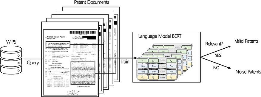
In two previous blog posts on my journey with BERT: Neural Search with BERT and Solr and Fun with Apache Lucene and BERT I’ve taken you through the practice of what it takes to enable semantic search powered by BERT in Solr (in fact, you can plug in any other dense embeddings method, other than BERT, as long as it outputs a float vector; a binary vector can also work). While it feels cool and modern to empower your search experience with a tech like BERT, making it performant is still important for productization. You want your search engine operations team to be happy in a real industrial setting. And you want your users to enjoy your search solution.
Devops cares about disk sizes, RAM and CPU consumption a lot. In some companies, they also care about electricity consumption. Scale for millions or billions of users and billions of documents is no cheap thing.
In Neural Search with BERT and Solr I did touch upon measuring time and memory consumption when dealing with BERT, with the time being both for indexing and search. And with indexing time there were some unpleasant surprises.
The search time is really a function of the number of documents, because from the algorithm complexity perspective it takes O(n), where n is the total number of documents in the index. This quickly becomes unwieldy, if you are indexing millions of docs and what’s even more important: you don’t really want to deliver n documents to your users: no one will have time to go through millions of documents in response to their searches. So why bother scoring all n? The reason why we need to visit all n documents is because we don’t know in advance which of these documents are going to correlate with the query in terms of dot-product or cosine distance between a document and query dense vectors.
In this blog post, I will apply the BERT dense embedding technique to Elasticsearch — a popular search engine of choice for many companies. We will look at implementing vanilla vector search and then will take a leap forward to KNN in vector search — measuring every step of our way.
Since there are plenty of blog posts talking about the intricacies of using vector search with Elasticsearch, I thought: what unique perspective could this blog post give you, my tireless reader? And this is what you will get today: I will share with you a substantially less known solution to handling vector search in Elasticsearch: using Associative Processing Unit (APU) implemented by GSI. I got a hold of this unique system that cares not only for the speed of querying vectors on large scale, but also for the amount of watts consumed (we do want to be eco-friendly to our Planet!). Sounds exciting? Let’s plunge in!
Elasticsearch’s own implementation of vector search
Elasticsearch is using Apache Lucene internally as a search engine, so many of the low-level concepts, data structures and algorithms (if not all) apply equally to Solr and Elasticsearch. Documented in https://www.elastic.co/blog/text-similarity-search-with-vectors-in-elasticsearch the approach to vector search has exactly the same limitation as what we observed with Solr: it will retrieve all documents that match the search criteria (keyword query along with filters on document attributes), and score all of them with the vector similarity of choice (cosine distance, dot-product or L1/L2 norms). That is, vector similarity will not be used during retrieval (first and expensive step): it will instead be used during document scoring (second step). Therefore, since you can’t know in advance, how many documents to fetch to surface most semantically relevant, the mathematical idea of vector search is not really applied.
Wait a sec, how is it different from TF-IDF or BM25 based search — why can’t we use the same trick with vector search? For BM25/TF-IDF algorithms you can precompute a bunch of information in the indexing phase to help during retrieval: term frequency, document frequency, document length and even a term position within the given document. Using these values, the scoring process can be applied during the retrieval step very efficiently. But you can’t apply cosine or dot-product similarities in the indexing phase: you don’t know what query your user will send your way, and hence can’t precompute the query embedding (except for some cases in e-commerce, where you can know this and therefore precompute everything).
But back to practice.
To run the indexer for vanilla Elasticsearch index, trigger the following command:
-time python src/index_dbpedia_abstracts_elastic.py
If you would like to reproduce the experiments, remember to alter the MAX_DOCS variable and set it to the desired number of documents to index.
As with every new tech, I’ve managed to run my Elasticsearch indexer code into an issue: the index became read-only during indexing process and would fail to advance! The reason is well explained here, in a nutshell: you need to ensure at least 5% of free disk space (51.5 gigabyte if you have a 1 TB disk!) in order to avoid this pesky issue or need to switch this safeguarding feature off (not recommended for production deployments).
The error looks like this:
{‘index’: {‘_index’: ‘vector’, ‘_type’: ‘_doc’, ‘_id’: ‘100’, ‘status’: 429, ‘error’: {‘type’: ‘cluster_block_exception’, ‘reason’: ‘index [vector] blocked by: [TOO_MANY_REQUESTS/12/disk usage exceeded flood-stage watermark, index has read-only-allow-delete block];’}
In this situation you can turn to Kibana — the UI tool, that grew from only data visualizations to security and index management, alerting and observability capabilities. For this blog post I’ve been routinely collecting index size information and inspecting index settings and mappings via index management dashboard:
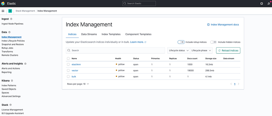
Index management dashboard for inspecting Elasticsearch index: health, docs count, storage size and whether the index is open for updates (Image by author)
If you still would like to get rid of this limitation , you can try something like this in Kibana Dev Tools (choose the suitable values for your use case — but be careful with the “cluster.routing.allocation.disk.watermark.flood_stage” value, since if it is too low, your OS might run into stability issues — consult official docs):
PUT _cluster/settings
{
   "transient":{
      "cluster.routing.allocation.disk.watermark.low":"100gb",
      "cluster.routing.allocation.disk.watermark.high":"50gb",
      "cluster.routing.allocation.disk.watermark.flood_stage":"10gb",
      "cluster.info.update.interval":"1m"
   }
}
After indexing, I’ve run 10 queries to measure the average speed. I’ve also recorded the time it took to index (including the time for computing vectors from text) and the size of the resulting index for each N=100, 200, 1000, 10000 and 20000. I did not record watt consumption, which could be an interesting idea for the next experiment.
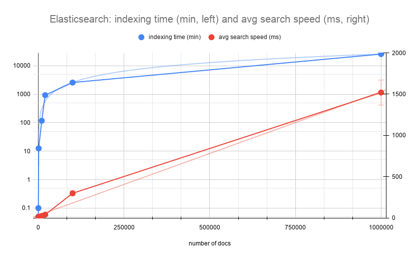
Indexing time vs search time as functions of number of documents (vanilla Elasticsearch, image by author)
Here is the raw table behind the chart above:
Since indexing was done with a single worker in bert-as-service, the indexing time grows exponentially, while the search speed advances sub-linearly to the number of documents. But how practical is this? For 20k short abstracts, 40ms for search seems to be too high. The index size grows linearly and that is a worrying factor as well (remember, that your devops teams can get concerned and you will need to prove the effectiveness of your algorithms).
Because it became impractical to index this slow, I had to find another way to compute vectors (most of the time goes to computing vectors, rather than to indexing them: I will prove it experimentally soon). So I took a look at Hugging Face library, that allows to index sentence embeddings using Siamese BERT-Networks, described here. In the case of Hugging Face, we also don’t need to use an http server, unlike in bert-as-service. Here is a sample code to get started:
from sentencetransformers import SentenceTransformersbert_model = SentenceTransformer('bert-base-nli-mean-tokens')def compute_sbert_vectors(text):
"""
Compute Sentence Embeddings using Siamese BERT-Networks: https://arxiv.org/abs/1908.10084 **:param** _text: single string with input text to compute embedding for :return: dense embeddings
numpy.ndarray or list[list[float]]
""" return sbert_model.encode([text])
SBERT approach managed to compute embeddings 6x faster, than bert-as-service. In practice, 1M vectors would take 18 days using bert-as-service and it took 3 days using SBERT with Hugging Face.
We can do better than O(n) in vector search
And the approach is to use a KNN algorithm to efficiently seek for document candidates in the closest vector sub-space.
I took 2 approaches that are available in the open source: elastiknn by Alex Klibisz and k-NN from Open Distro for Elasticsearch supported by AWS:
- https://github.com/alexklibisz/elastiknn
- https://github.com/opendistro-for-elasticsearch/k-NN
Let’s compare our vanilla vector search with these KNN methods on all three dimensions:
- indexing speed
- final index size
- search speed
KNN: elastiknn approach
We will first need to install the elastiknn plugin, that you can download from the project page:
bin/elasticsearch-plugin install file:////Users/dmitrykan/Desktop/Medium/Speeding_up_with_Elasticsearch/elastiknn/elastiknn-7.10.1.0.zip
To enable elastiknn on your index, you need to configure the following properties:
PUT /my-index
{
"settings": {
"index": {
"number_of_shards": 1, # 1
"elastiknn": true # 2
}
}
# 1 refers to the number of shards in your index, and sharding is the way to speed up the query, since it will be executed in parallel in each shard.
# 2 Elastiknn uses binary doc values for storing vectors. Setting this variable to true gives you significant speed improvements for Elasticsearch version ≥ 7.7, because it will prefer Lucene70DocValuesFormat with no compression of doc values over Lucene80DocValuesFormat, which uses compression, saving disk but increasing time for reading the doc values. It is worth to mention here, that Lucene80DocValuesFormat offers to trade compression ratio for better speed and vice versa starting Lucene 8.8 (relevant jira: https://issues.apache.org/jira/browse/LUCENE-9378, this version of Lucene is used in Elasticsearch 8.8.0-alpha1). So eventually these goodies will land both in Solr and Elasticsearch.
There are quite a few options for indexing and searching with different similarities — I recommend studying the well-written documentation.
To run the indexer for elastiknn index, trigger the following command:
time python src/index_dbpedia_abstracts_elastiknn.py
Indexing and search performance with elastiknn are summarized in the following table:
Performance of elastiknn, model: LSH, similarity: angular (L=99, k=1), top 10 candidates
KNN: Opendistro approach
I’ve run into many issues with Open Distro — and with this blog post I really hope to attract attention of OD developers, especially if you can find what can be improved in my configuration.
Without exaggeration I spent several days figuring out the maze of different settings to let OD index 1M vectors. My setup was:
- OD Elasticsearch running under docker: amazon/opendistro-for-elasticsearch:1.13.1
- Single node setup: kept only odfe-node1, no kibana
- opendistro_security.disabled=true
- “ES_JAVA_OPTS=-Xms4096m -Xmx4096m -XX:+UseG1GC -XX:G1ReservePercent=25 -XX:InitiatingHeapOccupancyPercent=30” # minimum and maximum Java heap size, recommend setting both to 50% of system RAM
- Sufficient disk size allocated for docker
I’ve also had index specific settings, and this is a suitable moment to show how to configure the KNN plugin:
"settings": {
"index": {
"knn": true, "knn.space_type": "cosinesimil", "refresh_interval": "-1", "merge.scheduler.max_thread_count": 1 }
}
Setting index.refresh_interval = 1 allows to avoid frequent index refresh to maximize for indexing throughput. And merge.scheduler.max_thread_count=1 restricts merging to a single thread to spend more resource on the indexing itself.
With these settings, I managed to index 200k documents into Open Distro Elasticsearch index. The important bit is to define the vector field like so:
"vector": {
"type": "knn_vector", "dimension": 768
}
The plugin builds Hierarchical Navigable Small World (HNSW) graphs during indexing, which are used to speed up KNN vector search. The graphs are built for each KNN field / Lucene segment pair, making it possible to efficiently find K nearest neighbours for the given query vector.
To run the indexer for Open Distro, trigger the following command:
time python src/index_dbpedia_abstracts_opendistro.py
To search, you need to wrap the query vector into the following object:
"size": docs_count,
"query": {
"knn": {
"vector": {
"vector": query_vector, "k": 10 }
}
}
Maximum k supported by the plugin is 10000. Each segment/shard will return k vectors, nearest to the query vector. Then the candidates will “roll up” to size number of resultant documents. Bear in mind, that if you use post filtering on the candidates, it may well be you get < k candidates per segment/shard, so it can also impact the final size.
The choice of KNN space type in the index settings defines the metric that will be used to find the K nearest neighbours. The “cosinesimil” setting corresponds to the following distance formula:
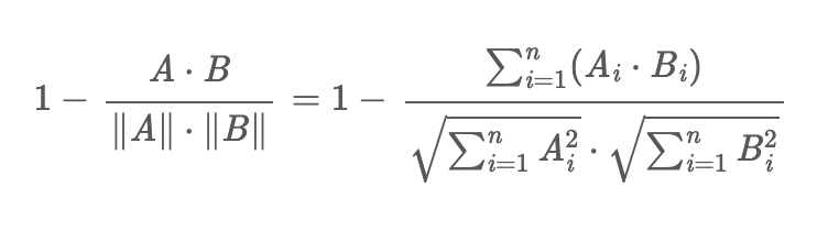
Distance function of “cosinesimil” space type (Screenshot from Open Distro)
From the plugin docs: “The cosine similarity formula does not include the 1 - prefix. However, because nmslib equates smaller scores with closer results, they return 1 - cosineSimilarity for their cosine similarity space—that’s why 1 - is included in the distance function.”
In KNN space, the smaller distance corresponds to closer vectors. This is opposite to how Elasticsearch scoring works: the higher score represents a more relevant result. To solve this, KNN plugin will turn the distance upside down into a 1 / (1 + distance) value.
I’ve run the measurements on indexing time, size and search speed, averaged across 10 queries (exactly the same queries were used for all the methods). Results:
Open Distro KNN performance, space type: cosinesimil
Making it even faster with GSI APU and Hugging Face
After two previous posts on BERT vector search in Solr and Lucene, I got contacted by GSI Technology and was offered to test their Elasticsearch plugin implementing distributed search powered by GSI’s Associative Processing Unit (APU) hardware technology. APU accelerates vector operations (like computing vector distance) and searches in-place directly in the memory array, instead of moving data back and forth between memory and CPU.
The architecture looks like this:
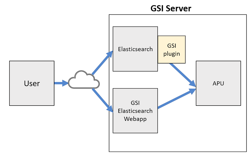
Architecture of the GSI APU powered Elasticsearch architecture (Screenshot provided by GSI Technology)
The query flow:
GSI query → Elasticsearch -> GSI plugin -> GSI server (APU) → top k of most relevant vectors → Elasticsearch → filter out → < ktopk=10 by default in single query and batch search
In order to use this solution, a user needs to produce two files:
- numpy 2D array with vectors of desired dimension (768 in my case)
- a pickle file with document ids matching the document ids of the said vectors in Elasticsearch.
After these data files get uploaded to the GSI server, the same data gets indexed in Elasticsearch. The APU powered search is performed on up to 3 Leda-G PCIe APU boards.
Since I’ve run into indexing performance with bert-as-service solution, I decided to take SBERT approach described above to prepare the numpy and pickle array files. This allowed me to index into Elasticsearch freely at any time, without waiting for days. You can use this script to do this on DBPedia data, which allows to choose between EmbeddingModel.HUGGING_FACE_SENTENCE (SBERT) and EmbeddingModel.BERT_UNCASED_768 (bert-as-service).
Next, I’ve precomputed 1M SBERT vector embeddings and fast-forward 3 days for vector embedding precomputation, I could index them into my Elasticsearch instance. I had to change the indexing script to parse the numpy&pickle files with 1M vectors and simultaneously read from DBPedia archive file to combine into a doc by doc indexing process. Then I’ve indexed 100k and 1M vectors into separate indexes to run my searches (10 queries for each).
For vanilla Elasticsearch 7.10.1 the results are as follows:
Elasticsearch 7.10.1 vanilla vector search performance
If we proportionally increase the time it would take to compute 1M vectors with bert-as-service approach to 25920 minutes, then SBERT approach is 17x faster! Index size is not going to change, because it depends on Lucene encoding and not on choosing BERT vs SBERT. Compacting the index size by reducing the vector precision is another interesting topic of research.
For elastiknn I got the following numbers:
Combining vanilla and elastiknn’s average speed metrics we get:
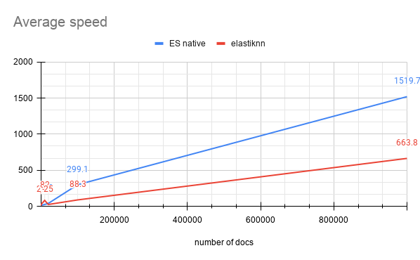
Elasticsearch vanilla vs elastiknn vector search performance (Image by author)
On my hardware elastiknn is 2,29x faster on average than Elasticsearch native vector search algorithm.
What about GSI APU solution? First, the indexing speed is not directly compatible with the above methods, because I had to separately produce the numpy+pickle files and upload them to GSI server. Indexing into Elasticsearch is comparable to what I did above and results in 15G index for 1M SBERT vectors. Next I ran the same 10 queries to measure the average speed. In order to run the queries with GSI Elasticsearch plugin, I needed to wrap query vector into the following query format:
Vector query format for GSI
Since I only uploaded 1M vectors, and experimented with 1M entries in the Elasticsearch index, I’ve got one number for the average speed over 10 queries: 92.6ms. This gives an upper bound on our speed graph for 1M mark on X axis:
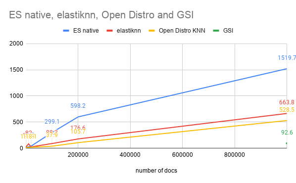
Average speed comparison between Elasticsearch native, elastiknn, Open Distro KNN and GSI APU vector search approaches (Image by author)
All times on this graph are from ‘took’ value reported by Elasticsearch. So none of these numbers include a network speed to transfer the results back to the client. However, the ‘took’ for GSI includes the communication between Elasticsearch and APU server.
What’s interesting is that GSI Elasticsearch plugin supports batch queries — this can be used for various use cases, for instance when you’d like to run several pre-crafted queries to get a data update on them. One specific use case could be creating user alerts on the queries of user interest — a very common use case for a number of commercial search engines.
To run a batch query, you will need to change the query like so:
In response, GSI plugin will execute queries in parallel and return you the top N (controlled with topK parameter) document ids for each query, with the cosine similarity:
The GSI’s search architecture scales to billions of documents. In this blog post, I have tested it with 1M DBPedia records and saw impressive results for performance.
Summary
I’ve studied 4 methods in this blog post, that can be grouped like so:
- Elasticsearch: vanilla (native) and elastiknn (external plugin)
- Open Distro KNN plugin
- GSI Elasticsearch plugin on top of APU
If you prefer to stay within the original Elasticsearch by Elastic, the best choice is elastiknn.
If you are open to Open Distro as the open source alternative to Elasticsearch by Elastic, you will win 50–150 ms. However, you might need extra help in setting things up.
If you like to try a commercial solution with hardware acceleration, then GSI plugin might be your choice, giving you comparatively the fastest vector query speed.
If you like to further explore the topics discussed in this blog post, read the next section, and leave a comment if you have something to ask or add.
Further reading on the topic
- Scripting your score in Elasticsearch (advanced math for vector search and much more): https://www.elastic.co/guide/en/elasticsearch/reference/7.6/query-dsl-script-score-query.html#vector-functions
- Chapter 3 “Finding Similar Items” that influenced the Random Projection algorithm in elastiknn used in this blog post: http://www.mmds.org/
- Performance evaluation of nearest neighbor search using Vespa, Elasticsearch and Open Distro for Elasticsearch K-NN: https://github.com/jobergum/dense-vector-ranking-performance/
- GSI Elasticsearch plugin: https://medium.com/gsi-technology/scalable-semantic-vector-search-with-elasticsearch-e79f9145ba8e
- Where Open Distro is heading: https://www.youtube.com/watch?v=J_6U1luNScg
- Non-Metric Space Library (NMSLIB): An efficient similarity search library and a toolkit for evaluation of k-NN methods for generic non-metric spaces: https://github.com/nmslib/nmslib/