Learn how to install OpenSearch Benchmark, create “workloads,” and benchmark them between computing devices​

OpenSearch users often want to know how their searches will perform in various environments, host types, and cluster configurations. OpenSearch Benchmark, a community-driven, open-source fork of Rally, is the ideal tool for that purpose.

OpenSearch-benchmark helps you to reduce infrastructure costs by optimizing OpenSearch resource usage. This tool also enables you to discover performance regressions and improve performance by running periodic benchmarks. Before benchmarking, you should try several other steps to improve performance — a subject I discussed in an earlier article.

In this article, I will lead you through setting up OpenSearch Benchmark and running search performance benchmarking comparing a widely used EC2 instance to a new computing accelerator — the Associative Processing Unit (APU) by Searchium.ai.

Step 1: Install Opensearch-benchmark​

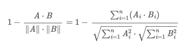
We’ll be using an m5.4xlarge (us-west-1) EC2 machine on which I installed OpenSearch and indexed a 9.1 M-sized vector index called laion_text. The index is a subset of the large laion dataset where I converted the text field to a vector representation (using a CLIP model):

Install Python 3.8+, including pip3, git 1.9+, and an appropriate JDK to run OpenSearch. Be sure that JAVA_HOME points to that JDK. Then run the following command:

sudo python3.8 -m pip install opensearch-benchmark

Tip: You might need to install each dependency manually.

• sudo apt install python3.8-dev
• sudo apt install python3.8-distutils
• python3.8 -m pip install multidict –upgrade
• python3.8 -m pip install attrs — upgrade
• python3.8 -m pip install yarl –upgrade
• python3.8 -m pip install async_timeout –upgrade
• python3.8 -m pip install aiosignal — upgrade

Run the following to verify that the installation was successful:

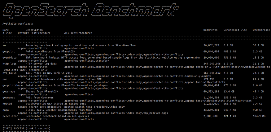
opensearch-benchmark list workloads

You should see the following details:

Step 2: Configure Where You Want Results To Be Saved​

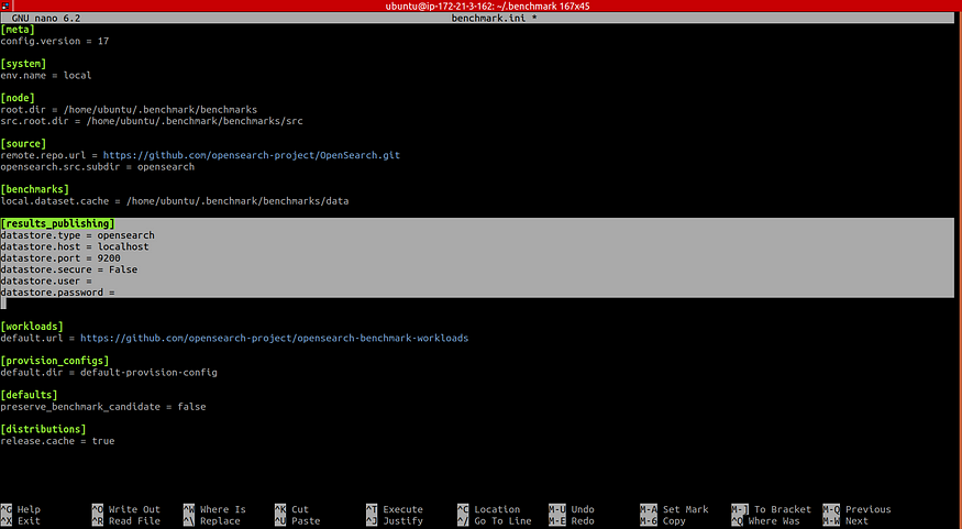
By default, OpenSearch Benchmark reports to “in-memory.” If set to “in-memory,” all metrics will be kept in memory while running the benchmark. If set to “opensearch,” all metrics will be written to a persistent metrics store, and the data will be available for further analysis.

To save the reported results in your OpenSearch cluster, open the opensearch-benchmark.ini file, which can be found in the ~/.benchmark folder and then modify the results publishing section in the highlighted area to write to the OpenSearch cluster:

Step 3: Construct the Search “Workload”​

Now that we have OpenSearch Benchmark installed properly, it’s time to start benchmarking!

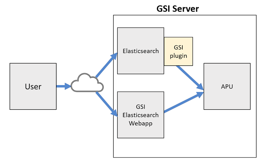
The plan is to use OpenSearch Benchmark to compare searches between two computing devices. You can use the following method to benchmark and compare any instance you wish. In this example, we will test a commonly used KNN flat search (an ANN example using IVF and HNSW will be covered in my next article) and compare an m5.4xlarge EC2 instance to the APU.

You can access the APU through a plugin downloaded from Searchium.ai’s SaaS platform. You can test the following benchmarking process on your own environment and data. A free trial is available, and registration is simple.

Each test/track in OpenSearch Benchmark is called a “workload.” We will create a workload for searching on the m5.4xlarge, which will act as our baseline. We will also create a workload for searching on the APU on the same EC2, which will act as our contender. Later, we will compare the performance of both workloads.

Let’s start by creating a workload for both the m5.4xlarge (CPU) and the APU using thelaion_text index (make sure you run these commands from within the .benchmark directory):

opensearch-benchmark create-workload --workload=laion_text_cpu --target-hosts=localhost:9200 --indices="laion_text”

opensearch-benchmark create-workload --workload=laion_text_apu --target-hosts=localhost:9200 --indices="laion_text”

Note: If the workloads are saved in a _workloads_ folder in your _home_ folder, you will need to copy them to the _.benchmark/benchmarks/workloads/default_ directory.

Run the opensearch-benchmark list workloads again and note that both laion_text_cpu and laion_text_apu are listed.

Next, we’ll add operations to the test schedule. You can add as many benchmarking tests as you want in this section. Add each test to the schedule in the workload.json file, which can be found in the folder with the index name you wish to benchmark.

In our case, it can be found in the following areas:

• ./benchmark/benchmarks/workloads/default/laion_text_apu
• ./benchmark/benchmarks/workloads/default/laion_text_cpu

We want to test out our OpenSearch search. Create an operation named “single vector search” (or any other name) and include a query vector. I cut out the vector itself because a 512 dimension vector would be a bit long… Add in the desired query vector and make sure to copy the same vector to the m5.4xlarge (CPU) and APU workload.json files!

Next, add any parameters you want. In this example, I will stick with the default eight clients and 1,000 iterations.

m5.4xlarge (CPU) workload.json:

{
   "schedule":[
      {
         "operation":{
            "name":"single-vector-search",
            "operation-type":"search",
            "body":{
               "size":"10",
               "query":{
                  "script_score":{
                     "query":{
                        "match_all":{
                           
                        }
                     },
                     "script":{
                        "source":"knn_score",
                        "lang":"knn",
                        "params":{
                           "field":"vector",
                           "query_value":[
                              "INSERT VECTOR HERE"
                           ],
                           "space_type":"cosinesimil"
                        }
                     }
                  }
               }
            }
         },
         "clients":8,
         "warmup-iterations":1000,
         "iterations":1000,
         "target-throughput":100
      }
   ]
}

APU workload.json:

{
  "schedule":[
    {
      "operation":{
        "name":"single-vector-search",
        "operation-type":"search",
        "body":{
          "size":"10",
          "query":{
            "gsi_knn":{
              "field":"vector",
              "vector":[
                "INSERT VECTOR HERE"
              ],
              "topk":"10"
            }
          }
        }
      },
      "clients":8,
      "warmup-iterations":1000,
      "iterations":1000,
      "target-throughput":100
    }
  ]
}

Step 4: Run our Workloads​

It’s time to run our workloads! We are interested in running our search workloads on a running OpenSearch cluster. I added a few parameters to the execute_test command:

Distribution-version — Make sure to add your correct OpenSearch version.

Workload — Our workload name.

Other parameters are available. I added the pipeline, client-options, and on-error, which simplifies the whole process.

Go ahead and run the following commands, which will run our workloads:

opensearch-benchmark execute_test --distribution-version=2.2.0 --workload=laion_text_apu --pipeline=benchmark-only --client-options=verify_certs:false,use_ssl:false --on-error=abort --client-options="timeout:320"

opensearch-benchmark execute_test --distribution-version=2.2.0 --workload=laion_text_cpu --pipeline=benchmark-only --client-options=verify_certs:false,use_ssl:false --on-error=abort --client-options="timeout:320"

And now we wait…

Bonus benchmark: I was interested to see the results on an Arm-based Amazon Graviton2 processor, so I ran the same exact process on an r6g.8xlarge EC2 as well.

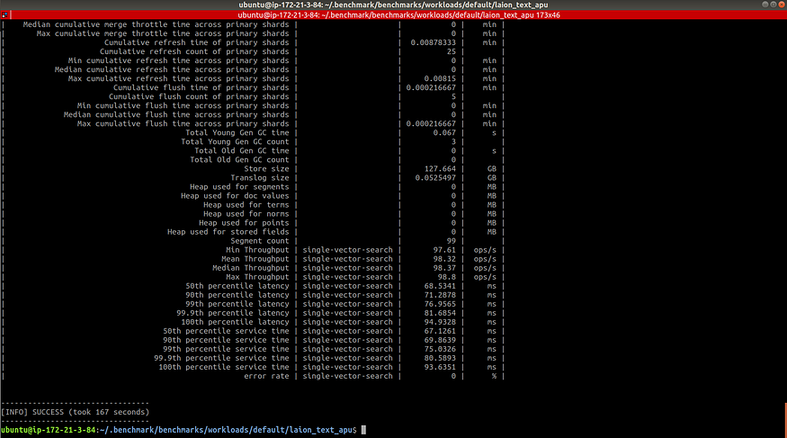
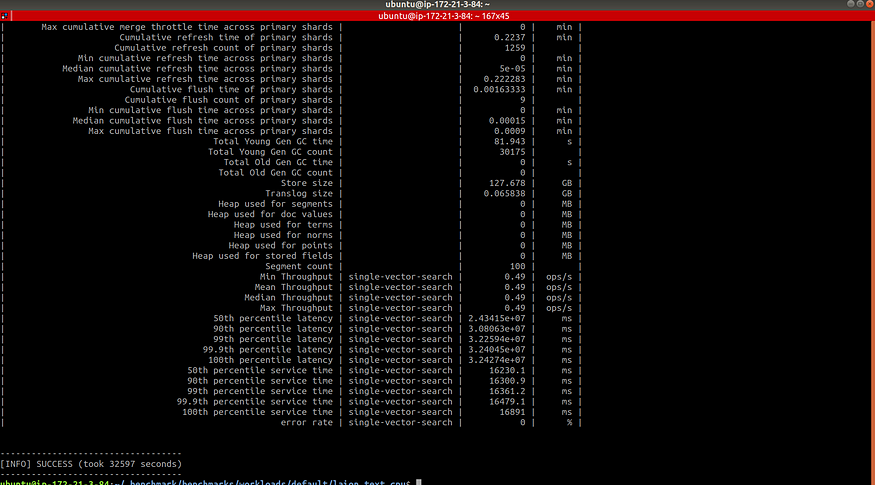
Our results should look like the following:

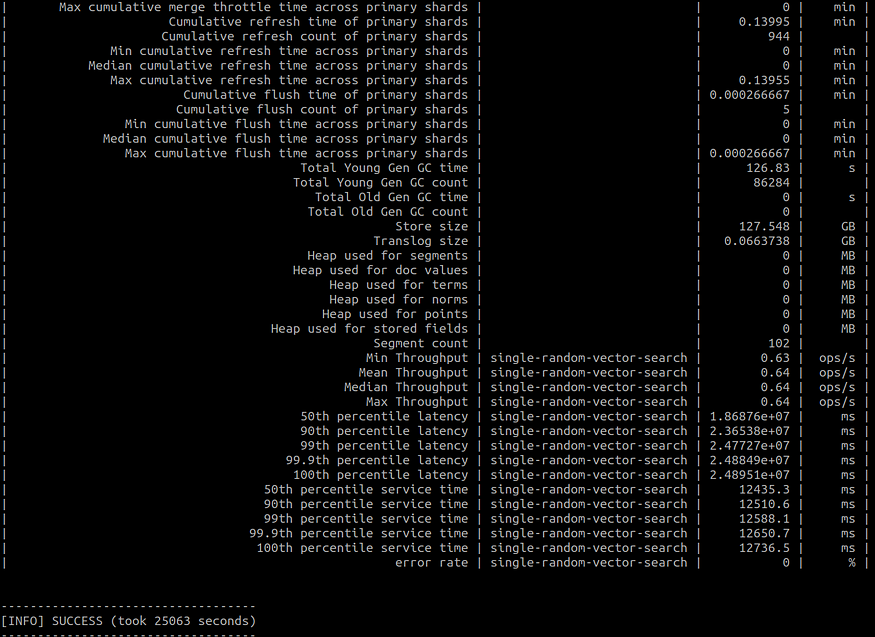
Step 5: Compare our Results​

We are finally ready to look at our test results. Drumroll, please… 🥁

First, we noticed the running times of each workload were different. The m5.4xlarge workload took 9 hours, and the r6g.8xlarge workload took 6.96 hours, while the APU workload took 2.78 minutes. This is because the APU also supports query aggregation, allowing for greater throughput.

Now, we want a more comprehensive comparison between our workloads. OpenSearch Benchmark enables us to generate a CSV file where we can scompare between workloads easily.

First, we will need to find the workload IDs for each case. This can be done by either looking in the OpenSearch benchmark-test-executions index (which was created in step 2) or in the benchmarks folder:

Using the workloads IDs, run the following command to compare two workloads and display the output in a CSV file:

opensearch-benchmark compare --results-format=csv --show-in-results=search --results-file=data.csv --baseline=ecb4af7a-d53c-4ac3-9985-b5de45daea0d --contender=b714b13a-af8e-4103-a4c6-558242b8fe6a

Here’s a short summary comparing three of our workload results:

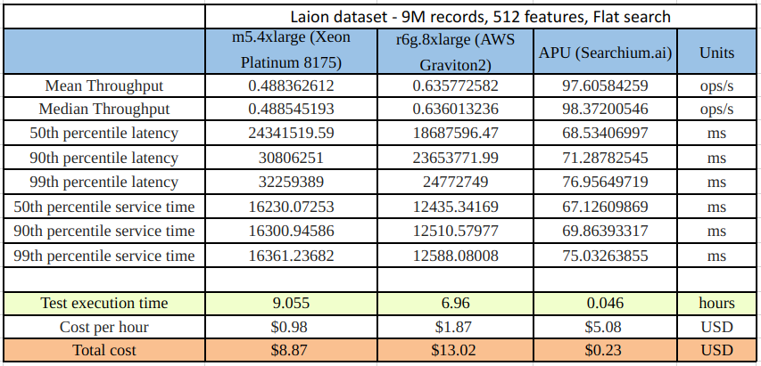
A brief explanation of the results in the table:

1. Throughput: The number of operations that OpenSearch can perform within a certain period, usually per second.

2. Latency: The time between submitting a request and receiving the complete response. It also includes wait time, i.e., the time the request spends waiting until it is ready to be serviced by OpenSearch.

3. Service time: The time between sending a request and receiving the corresponding response. This metric can easily be confused with latency but does not include waiting time. This is what most load testing tools incorrectly refer to as “latency.”

4. Test execution time: The total runtime from starting the workload until completion.

Conclusion​

When looking at our results, we can see that the service time for the APU workload was 197 times faster than the m5.4xlarge workload and 151 times faster then the r6g.8xlarge. From a cost perspective, running the same workload on the APU costs $0.23 as opposed to $8.87 on the m5.4xlarge (38 times less expensive) and $13.02 on the r6g.8xlarge (56 times less expensive), and we got our search results almost 9 hours (m5.4xlarge) and 6.91 hours (r6g.8xlarge) earlier.

Now, imagine the magnitude of these benefits when scaling to even larger datasets, which is likely to be the case in our data-driven, fast-paced world.

I hope this helped you understand more about the power of OpenSearch’s benchmarking tool and how you can use it to benchmark your search performance.

For more information about Searchium.ai’s plugin and the APU, please visit www.searchium.ai. They even offer a free trial!

Natural language processing (NLP) is a major part of search — so much so that it is even being used in image search applications.

For example, Google said, when talking about its MUM model, “Eventually, you might be able to take a photo of your hiking boots and ask, ‘can I use these to hike Mt. Fuji?’ MUM would understand the image and connect it with your question to let you know your boots would work just fine. It could then point you to a blog with a list of recommended gear.” This makes MUM multimodal because it understands both text and images.

In this post, I’ll show how vector embeddings outperform keyword search for multimodal text-to-image search. I’ll also discuss a solution that allows you to leverage your existing OpenSearch installation to quickly and easily create a text-to-image search application.

The Limitations of Keyword Search​

Previously, when using text to search for relevant images, one would perform keyword search using the image captions to compare against the text query. This meant the image itself wasn’t even being used in the search.

One problem with this is there could be relevant images that don’t have captions. This could result in the images not being returned as candidates, even though they are relevant.

Another problem with keyword search is it could omit images with captions that don’t share many keywords with the query but are in fact relevant images. This could impact business in e-commerce applications because sellers often don’t enter the most descriptive text, so even if their item is exactly what the buyer is looking for, it might not be returned as a candidate.

Also, as shown in this post, keyword search has limited understanding of user intent and could return irrelevant images even if there are “multiple matching terms between the query and the result.” As shown below, it incorrectly returned an image where the caption matched the keywords eating fish, but it missed the main search term bear.

Query: A bear eating fish by a river

Result: heron eating fish

An irrelevant search result returned using keyword search for the query “A bear eating fish by a river.” Source

Vector Embeddings — The Key to Text-to-Image Search​

To address the previously mentioned keyword search limitations, we can use a multilingual CLIP model to generate vector embeddings. CLIP was created by OpenAI, and they state that it “efficiently learns visual concepts from natural language supervision.” Basically, CLIP maps text and images to the same embedding space where they can be compared for similarity.

As we discussed in a previous post, vector embeddings better understand the searcher’s intent and the contextual meaning of the query. Instead of simply matching the keywords, it takes into consideration what the words mean and not just the words themselves.

An example of that can be seen in the image below. In this case, vector embeddings were used instead of keywords. The same query about a bear eating a fish was used, but unlike the keyword approach that returned an irrelevant image, vector embeddings returned a relevant image.

A relevant search result using vector embeddings for the query “nehir kenarında balık yiyen ayı” (a bear eating fish by a river — Turkish)

Not only did vector embedding return a relevant image, but the vector embeddings approach also showed that it understands multiple languages, in this example, Turkish.

Vector embeddings can also improve recall. Recall is important because it can impact a company’s business. For example, in e-commerce, sellers often either don’t enter very descriptive text, don’t use the right keywords, or they might enter incorrect text descriptions. In these cases, keyword search could prevent a product from being returned as a match, even if it actually is. This means a missed business opportunity for the seller.

Vector embeddings address this recall issue because even though the text descriptions were poor in those examples above, if there were relevant images that went with them, the vector embeddings of the images would allow those images to be returned as matches. Thus, the seller is no longer penalized for entering poor product descriptions, or even no descriptions.

Easily Add Vector Embedding Search to Your OpenSearch​

As we wrote about in this post, GSI Technology’s OpenSearch k-NN plugin allows users to easily add production-grade vector embedding search to their search pipeline. They can leverage their current OpenSearch installation rather than having to learn new software for one of the other vector search options out there. This saves them valuable time and resources.

Dmitry Kan and Aarne Talman recently published a great blog post where they explained how they used our OpenSearch k-NN plugin as part of their search stack to easily create a text-to-image search application.

In addition to saving developers valuable time and resources, our OpenSearch k-NN plugin allows for billion-scale neural search and addresses one of the key limitations of native OpenSearch — namely it’s lack of pre-filter support for nearest neighbor vector search.

Pre-filtering on metadata is used in many search applications. For example, product metadata such as item description, item title, category, color, or brand are often used as pre-filters to a search query.

The OpenSearch website states: “Because the native library indices are constructed during indexing, it is not possible to apply a filter on an index and then use this search method. All filters are applied on the results produced by the approximate nearest neighbor search.” This means that native OpenSearch only supports post-filtering of the approximate nearest neighbor results and doesn’t support pre-filtering

As mentioned in one of our previous posts, post-filtering is problematic because it has a high likelihood of returning far fewer results than the intended k-nearest neighbors. In fact, it could lead to zero results being returned. This leads to an unsatisfying user experience since very few, or no, relevant results might be returned for a particular search query.

GSI’s OpenSearch plugin supports pre-filtering, and even supports range filtering. For example, if somebody was searching for shirts, in addition to using common filters such as brand, style, size, and color, they could also add a range filter, for example, to limit the search to shirts in the range between $55 and $85.

Summary​

This post showed some of the advantages of vector embedding search over keyword search — for example, better understanding user intent and improving recall in e-commerce applications where sellers either don’t enter very descriptive text, don’t use the right keywords, or enter incorrect text descriptions. Ultimately, these vector embedding advantages lead to improved business for sellers.

We also presented our OpenSearch k-NN plugin that allows users to easily add production-grade vector embedding search to their search pipeline — saving them valuable time and resources. The plugin also provides billion-scale search along with strong filtering capability.

If you want to try out our OpenSearch k-NN plugin, please contact us at opensearch@gsitechnology.com.

Neural search (also commonly referred to as vector search or semantic search) is hot — it seems like almost every day I see a new article written about it. For example, I recently saw these articles from Google, Home Depot, and Spotify.

That’s why I shouldn’t be too surprised by the number of people who have reached out to us to see if our Elasticsearch and OpenSearch k-NN plugins can accelerate their neural search applications.

In this post, I’ll briefly present a few of those applications, many of which need to search through large amounts of unstructured data — ranging from hundreds of millions to billions of items.

The Move to Neural Search

Traditional search engines use an inverted index along with something like TF-IDF or BM25 for ranking. They use sparse vectors, based on literal keywords, to find similar/relevant information.

As we wrote about in a previous blog post, these traditional approaches are limited in their understanding of user intent. For example, they could omit documents that don’t share many keywords with the query but are relevant documents.

Search is moving beyond this simple keyword-based search, to neural search, where user intent is better captured.

Neural search uses neural networks to better understand user intent and go beyond traditional exact-match keyword search.

Neural Search Applications

Here are just a few of the neural search applications that people have talked to us about:

Prior Art Search​

Traditionally, IP experts have spent a lot of time analyzing documents to come up with relevant keywords for a prior art patent search. Some of the keywords can be very subtle and can be missed if done manually.

Also, with datasets in this space growing rapidly, oftentimes in the billions of documents, relying solely on human analysis is not realistic or scalable.

That’s why IP experts are turning to neural search to efficiently sift through those billions of documents. Neural search provides the ability to quickly search through patent data by focusing on context, and not just keywords, to provide relevant references.

Figure 1 below is an example from a paper that shows how neural search can be used in prior art discovery.

Figure 1. Neural search in prior art discovery. A language model is used to compare embeddings of a query to embeddings from patent documents to determine if a patent is relevant. (source: Patent prior art search using deep learning language model)

Recruitment and Talent Acquisition​

In this application, candidates and job descriptions are mapped to a common embedding space to find potential fits. This can be used to recommend and rank candidates for a particular position, find similar candidates, or to find similar positions.

This application typically has large data requirements, on the order of hundreds of millions of documents.

Semantic Video Transcription​

Have you ever experienced the frustration of watching a video and later wanted to find a specific topic in the video, but you couldn’t remember exactly where it was in the video? If so, then video transcription with semantic search can save you from having to sift through the whole video to find it.

Basically, what this application does is break the transcribed video down into paragraphs that are semantically indexed. A neural search between the query and this semantically indexed content then helps you find what you’re looking for.

Targeted Advertising​

This is where companies like Google and Facebook analyze online behavior to categorize individuals. They then use this information to match groups of finely categorized people to individualized advertisements — creating a targeted advertisement. This is done by creating embeddings for target customers and advertisements and mapping them to a common embedding space such that a similarity search can be performed to find the right match.

Your Applications

If you’re using neural search in your application, I’d love for you to share a bit about it in the comments section.

Also, if you would like to see if our Elasticsearch or OpenSearch plugins can help accelerate your neural search application, please contact us at elasticsearch@gsitechnology.com.

Photo by Benjamin Wedemeyer on Unsplash

Neural Search — Taking the Leap from Keyword Search

Semantic vector search is a topic that’s getting a lot of attention, and many search developers are wondering if, and how, they should add it to their search solution.

In a recent Haystack LIVE! Meetup titled Evolving from Keyword to Neural Search,

Branden Chan

of Deepset presented their Haystack NLP framework and was asked what approach he would recommend for adding semantic vector search to a platform based on bag-of-words (keyword) search.

In this post, I will review Branden’s recommendation and propose a way to implement his proposal.

Traditional Search​

Traditional search engines, like Elasticsearch, rely heavily on a bag-of-words (keyword) approach that uses an inverted index along with TF-IDF or BM25 ranking functions. A sparse vector, based on literal keyword matching, is used to find similar/relevant information.

As we wrote about in a previous blog post, this keyword approach has some limitations in terms of understanding user intent. For example, it could omit documents that don’t share many keywords with the query but are relevant documents.

Combining Keyword and Semantic Search​

Recognizing these limitations, many search developers have been wondering if they should add dense vector semantic search to their platform to better capture user intent. In fact, one of the attendees of Branden Chan’s recent talk titled Evolving from Keyword to Neural Search asked Braden for his thoughts about that.

The attendee mentioned that they have a content server, and they are currently using a bag-of-words (BoW) approach for search. They said that sometimes their users know exactly what they’re searching for, but other times their search is exploratory and, in that case, if you’re limited to a BoW approach, it’s hard to understand exactly what the user wants.

He said that he is interested in seeing if dense vectors could help him better understand user intent. He mentioned that he couldn’t switch to a dense vector solution “overnight,” due to implementation reasons and concerns of how it could change performance over time. He was interested in Branden’s advice on how to incrementally take advantage of dense vector search to make search better.

Branden said that you could use the existing sparse (keyword) score and combine it with a dense (semantic) vector score. He suggested passing the query to both a dense and sparse path, with each path having a score that you could weight.

Branden said you could take a cautious path of lightly weighting the dense score initially and then incrementally bumping it up and experimenting to see how to optimally weight it.

How to Add Semantic Search Incrementally​

One way a user could implement Branden’s incremental approach is to use one of our Elasticsearch or OpenSearch k-NN plugins along with the user’s current Elasticsearch or OpenSearch installations.

That would allow the user to leverage the powerful keyword search (sparse vector) capabilities of Elasticsearch and OpenSearch and combine it with semantic vector search (dense vector) of one of GSI’s k-NN plugins.

Installing the plugins is easy, and they allow for vector similarity search to be run as simply as any standard Elasticsearch query. The Elasticsearch k-NN plugin provides similarity search results in the standard Elasticsearch format, so a user could follow Branden’s advice of combining the sparse and dense vector scores. The user could lightly weight the dense score (k-NN result) initially and then incrementally bump it up and experiment to see how to optimally weight it.

For more information about GSI’s k-NN plugins, contact us at elasticsearch@gsitechnology.com.

Neural Search in Elasticsearch: from vanilla to KNN to hardware acceleration​

BERT (Image via Flickr, licensed under CC BY-SA 2.0 / background blurred by author)

In two previous blog posts on my journey with BERT: Neural Search with BERT and Solr and Fun with Apache Lucene and BERT I’ve taken you through the practice of what it takes to enable semantic search powered by BERT in Solr (in fact, you can plug in any other dense embeddings method, other than BERT, as long as it outputs a float vector; a binary vector can also work). While it feels cool and modern to empower your search experience with a tech like BERT, making it performant is still important for productization. You want your search engine operations team to be happy in a real industrial setting. And you want your users to enjoy your search solution.

Devops cares about disk sizes, RAM and CPU consumption a lot. In some companies, they also care about electricity consumption. Scale for millions or billions of users and billions of documents is no cheap thing.

In Neural Search with BERT and Solr I did touch upon measuring time and memory consumption when dealing with BERT, with the time being both for indexing and search. And with indexing time there were some unpleasant surprises.

The search time is really a function of the number of documents, because from the algorithm complexity perspective it takes O(n), where n is the total number of documents in the index. This quickly becomes unwieldy, if you are indexing millions of docs and what’s even more important: you don’t really want to deliver n documents to your users: no one will have time to go through millions of documents in response to their searches. So why bother scoring all n? The reason why we need to visit all n documents is because we don’t know in advance which of these documents are going to correlate with the query in terms of dot-product or cosine distance between a document and query dense vectors.

In this blog post, I will apply the BERT dense embedding technique to Elasticsearch — a popular search engine of choice for many companies. We will look at implementing vanilla vector search and then will take a leap forward to KNN in vector search — measuring every step of our way.

Since there are plenty of blog posts talking about the intricacies of using vector search with Elasticsearch, I thought: what unique perspective could this blog post give you, my tireless reader? And this is what you will get today: I will share with you a substantially less known solution to handling vector search in Elasticsearch: using Associative Processing Unit (APU) implemented by GSI. I got a hold of this unique system that cares not only for the speed of querying vectors on large scale, but also for the amount of watts consumed (we do want to be eco-friendly to our Planet!). Sounds exciting? Let’s plunge in!

Elasticsearch’s own implementation of vector search

Elasticsearch is using Apache Lucene internally as a search engine, so many of the low-level concepts, data structures and algorithms (if not all) apply equally to Solr and Elasticsearch. Documented in https://www.elastic.co/blog/text-similarity-search-with-vectors-in-elasticsearch the approach to vector search has exactly the same limitation as what we observed with Solr: it will retrieve all documents that match the search criteria (keyword query along with filters on document attributes), and score all of them with the vector similarity of choice (cosine distance, dot-product or L1/L2 norms). That is, vector similarity will not be used during retrieval (first and expensive step): it will instead be used during document scoring (second step). Therefore, since you can’t know in advance, how many documents to fetch to surface most semantically relevant, the mathematical idea of vector search is not really applied.

Wait a sec, how is it different from TF-IDF or BM25 based search — why can’t we use the same trick with vector search? For BM25/TF-IDF algorithms you can precompute a bunch of information in the indexing phase to help during retrieval: term frequency, document frequency, document length and even a term position within the given document. Using these values, the scoring process can be applied during the retrieval step very efficiently. But you can’t apply cosine or dot-product similarities in the indexing phase: you don’t know what query your user will send your way, and hence can’t precompute the query embedding (except for some cases in e-commerce, where you can know this and therefore precompute everything).

But back to practice.

To run the indexer for vanilla Elasticsearch index, trigger the following command:

-time python src/index_dbpedia_abstracts_elastic.py

If you would like to reproduce the experiments, remember to alter the MAX_DOCS variable and set it to the desired number of documents to index.

As with every new tech, I’ve managed to run my Elasticsearch indexer code into an issue: the index became read-only during indexing process and would fail to advance! The reason is well explained here, in a nutshell: you need to ensure at least 5% of free disk space (51.5 gigabyte if you have a 1 TB disk!) in order to avoid this pesky issue or need to switch this safeguarding feature off (not recommended for production deployments).

The error looks like this:

{‘index’: {‘_index’: ‘vector’, ‘_type’: ‘_doc’, ‘_id’: ‘100’, ‘status’: 429, ‘error’: {‘type’: ‘cluster_block_exception’, ‘reason’: ‘index [vector] blocked by: [TOO_MANY_REQUESTS/12/disk usage exceeded flood-stage watermark, index has read-only-allow-delete block];’}

In this situation you can turn to Kibana — the UI tool, that grew from only data visualizations to security and index management, alerting and observability capabilities. For this blog post I’ve been routinely collecting index size information and inspecting index settings and mappings via index management dashboard:

Index management dashboard for inspecting Elasticsearch index: health, docs count, storage size and whether the index is open for updates (Image by author)

If you still would like to get rid of this limitation , you can try something like this in Kibana Dev Tools (choose the suitable values for your use case — but be careful with the “cluster.routing.allocation.disk.watermark.flood_stage” value, since if it is too low, your OS might run into stability issues — consult official docs):

PUT _cluster/settings
{
   "transient":{
      "cluster.routing.allocation.disk.watermark.low":"100gb",
      "cluster.routing.allocation.disk.watermark.high":"50gb",
      "cluster.routing.allocation.disk.watermark.flood_stage":"10gb",
      "cluster.info.update.interval":"1m"
   }
}

After indexing, I’ve run 10 queries to measure the average speed. I’ve also recorded the time it took to index (including the time for computing vectors from text) and the size of the resulting index for each N=100, 200, 1000, 10000 and 20000. I did not record watt consumption, which could be an interesting idea for the next experiment.

Indexing time vs search time as functions of number of documents (vanilla Elasticsearch, image by author)

Here is the raw table behind the chart above:

Since indexing was done with a single worker in bert-as-service, the indexing time grows exponentially, while the search speed advances sub-linearly to the number of documents. But how practical is this? For 20k short abstracts, 40ms for search seems to be too high. The index size grows linearly and that is a worrying factor as well (remember, that your devops teams can get concerned and you will need to prove the effectiveness of your algorithms).

Because it became impractical to index this slow, I had to find another way to compute vectors (most of the time goes to computing vectors, rather than to indexing them: I will prove it experimentally soon). So I took a look at Hugging Face library, that allows to index sentence embeddings using Siamese BERT-Networks, described here. In the case of Hugging Face, we also don’t need to use an http server, unlike in bert-as-service. Here is a sample code to get started:

from sentencetransformers import SentenceTransformersbert_model = SentenceTransformer('bert-base-nli-mean-tokens')def compute_sbert_vectors(text):
"""
Compute Sentence Embeddings using Siamese BERT-Networks: https://arxiv.org/abs/1908.10084 **:param** _text: single string with input text to compute embedding for :return: dense embeddings
numpy.ndarray or list[list[float]]
""" return sbert_model.encode([text])

SBERT approach managed to compute embeddings 6x faster, than bert-as-service. In practice, 1M vectors would take 18 days using bert-as-service and it took 3 days using SBERT with Hugging Face.

We can do better than O(n) in vector search

And the approach is to use a KNN algorithm to efficiently seek for document candidates in the closest vector sub-space.

I took 2 approaches that are available in the open source: elastiknn by Alex Klibisz and k-NN from Open Distro for Elasticsearch supported by AWS:

1. https://github.com/alexklibisz/elastiknn
2. https://github.com/opendistro-for-elasticsearch/k-NN

Let’s compare our vanilla vector search with these KNN methods on all three dimensions:

• indexing speed
• final index size
• search speed

KNN: elastiknn approach

We will first need to install the elastiknn plugin, that you can download from the project page:

bin/elasticsearch-plugin install file:////Users/dmitrykan/Desktop/Medium/Speeding_up_with_Elasticsearch/elastiknn/elastiknn-7.10.1.0.zip

To enable elastiknn on your index, you need to configure the following properties:

PUT /my-index
{
"settings": {
"index": {
"number_of_shards": 1, # 1
"elastiknn": true # 2

}  

}
}

# 1 refers to the number of shards in your index, and sharding is the way to speed up the query, since it will be executed in parallel in each shard.

# 2 Elastiknn uses binary doc values for storing vectors. Setting this variable to true gives you significant speed improvements for Elasticsearch version ≥ 7.7, because it will prefer Lucene70DocValuesFormat with no compression of doc values over Lucene80DocValuesFormat, which uses compression, saving disk but increasing time for reading the doc values. It is worth to mention here, that Lucene80DocValuesFormat offers to trade compression ratio for better speed and vice versa starting Lucene 8.8 (relevant jira: https://issues.apache.org/jira/browse/LUCENE-9378, this version of Lucene is used in Elasticsearch 8.8.0-alpha1). So eventually these goodies will land both in Solr and Elasticsearch.

There are quite a few options for indexing and searching with different similarities — I recommend studying the well-written documentation.

To run the indexer for elastiknn index, trigger the following command:

time python src/index_dbpedia_abstracts_elastiknn.py

Indexing and search performance with elastiknn are summarized in the following table:

Performance of elastiknn, model: LSH, similarity: angular (L=99, k=1), top 10 candidates

KNN: Opendistro approach

I’ve run into many issues with Open Distro — and with this blog post I really hope to attract attention of OD developers, especially if you can find what can be improved in my configuration.

Without exaggeration I spent several days figuring out the maze of different settings to let OD index 1M vectors. My setup was:

1. OD Elasticsearch running under docker: amazon/opendistro-for-elasticsearch:1.13.1
2. Single node setup: kept only odfe-node1, no kibana
3. opendistro_security.disabled=true
4. • “ES_JAVA_OPTS=-Xms4096m -Xmx4096m -XX:+UseG1GC -XX:G1ReservePercent=25 -XX:InitiatingHeapOccupancyPercent=30” # minimum and maximum Java heap size, recommend setting both to 50% of system RAM
5. Sufficient disk size allocated for docker

I’ve also had index specific settings, and this is a suitable moment to show how to configure the KNN plugin:

"settings": {
"index": {
"knn": true, "knn.space_type": "cosinesimil", "refresh_interval": "-1", "merge.scheduler.max_thread_count": 1 }
}

Setting index.refresh_interval = 1 allows to avoid frequent index refresh to maximize for indexing throughput. And merge.scheduler.max_thread_count=1 restricts merging to a single thread to spend more resource on the indexing itself.

With these settings, I managed to index 200k documents into Open Distro Elasticsearch index. The important bit is to define the vector field like so:

"vector": {
"type": "knn_vector", "dimension": 768
}

The plugin builds Hierarchical Navigable Small World (HNSW) graphs during indexing, which are used to speed up KNN vector search. The graphs are built for each KNN field / Lucene segment pair, making it possible to efficiently find K nearest neighbours for the given query vector.

To run the indexer for Open Distro, trigger the following command:

time python src/index_dbpedia_abstracts_opendistro.py

To search, you need to wrap the query vector into the following object:

"size": docs_count,
"query": {
"knn": {
"vector": {
"vector": query_vector, "k": 10 }
}
}

Maximum k supported by the plugin is 10000. Each segment/shard will return k vectors, nearest to the query vector. Then the candidates will “roll up” to size number of resultant documents. Bear in mind, that if you use post filtering on the candidates, it may well be you get < k candidates per segment/shard, so it can also impact the final size.

The choice of KNN space type in the index settings defines the metric that will be used to find the K nearest neighbours. The “cosinesimil” setting corresponds to the following distance formula:

Distance function of “cosinesimil” space type (Screenshot from Open Distro)

From the plugin docs: “The cosine similarity formula does not include the 1 - prefix. However, because nmslib equates smaller scores with closer results, they return 1 - cosineSimilarity for their cosine similarity space—that’s why 1 - is included in the distance function.”

In KNN space, the smaller distance corresponds to closer vectors. This is opposite to how Elasticsearch scoring works: the higher score represents a more relevant result. To solve this, KNN plugin will turn the distance upside down into a 1 / (1 + distance) value.

I’ve run the measurements on indexing time, size and search speed, averaged across 10 queries (exactly the same queries were used for all the methods). Results:

Open Distro KNN performance, space type: cosinesimil

Making it even faster with GSI APU and Hugging Face

After two previous posts on BERT vector search in Solr and Lucene, I got contacted by GSI Technology and was offered to test their Elasticsearch plugin implementing distributed search powered by GSI’s Associative Processing Unit (APU) hardware technology. APU accelerates vector operations (like computing vector distance) and searches in-place directly in the memory array, instead of moving data back and forth between memory and CPU.

The architecture looks like this:

Architecture of the GSI APU powered Elasticsearch architecture (Screenshot provided by GSI Technology)

The query flow:

GSI query → Elasticsearch -> GSI plugin -> GSI server (APU) → top k of most relevant vectors → Elasticsearch → filter out → < ktopk=10 by default in single query and batch search

In order to use this solution, a user needs to produce two files:

• numpy 2D array with vectors of desired dimension (768 in my case)
• a pickle file with document ids matching the document ids of the said vectors in Elasticsearch.

After these data files get uploaded to the GSI server, the same data gets indexed in Elasticsearch. The APU powered search is performed on up to 3 Leda-G PCIe APU boards.

Since I’ve run into indexing performance with bert-as-service solution, I decided to take SBERT approach described above to prepare the numpy and pickle array files. This allowed me to index into Elasticsearch freely at any time, without waiting for days. You can use this script to do this on DBPedia data, which allows to choose between EmbeddingModel.HUGGING_FACE_SENTENCE (SBERT) and EmbeddingModel.BERT_UNCASED_768 (bert-as-service).

Next, I’ve precomputed 1M SBERT vector embeddings and fast-forward 3 days for vector embedding precomputation, I could index them into my Elasticsearch instance. I had to change the indexing script to parse the numpy&pickle files with 1M vectors and simultaneously read from DBPedia archive file to combine into a doc by doc indexing process. Then I’ve indexed 100k and 1M vectors into separate indexes to run my searches (10 queries for each).

For vanilla Elasticsearch 7.10.1 the results are as follows:

Elasticsearch 7.10.1 vanilla vector search performance

If we proportionally increase the time it would take to compute 1M vectors with bert-as-service approach to 25920 minutes, then SBERT approach is 17x faster! Index size is not going to change, because it depends on Lucene encoding and not on choosing BERT vs SBERT. Compacting the index size by reducing the vector precision is another interesting topic of research.

For elastiknn I got the following numbers:

Combining vanilla and elastiknn’s average speed metrics we get:

Elasticsearch vanilla vs elastiknn vector search performance (Image by author)

On my hardware elastiknn is 2,29x faster on average than Elasticsearch native vector search algorithm.

What about GSI APU solution? First, the indexing speed is not directly compatible with the above methods, because I had to separately produce the numpy+pickle files and upload them to GSI server. Indexing into Elasticsearch is comparable to what I did above and results in 15G index for 1M SBERT vectors. Next I ran the same 10 queries to measure the average speed. In order to run the queries with GSI Elasticsearch plugin, I needed to wrap query vector into the following query format:

Vector query format for GSI

Since I only uploaded 1M vectors, and experimented with 1M entries in the Elasticsearch index, I’ve got one number for the average speed over 10 queries: 92.6ms. This gives an upper bound on our speed graph for 1M mark on X axis:

Average speed comparison between Elasticsearch native, elastiknn, Open Distro KNN and GSI APU vector search approaches (Image by author)

All times on this graph are from ‘took’ value reported by Elasticsearch. So none of these numbers include a network speed to transfer the results back to the client. However, the ‘took’ for GSI includes the communication between Elasticsearch and APU server.

What’s interesting is that GSI Elasticsearch plugin supports batch queries — this can be used for various use cases, for instance when you’d like to run several pre-crafted queries to get a data update on them. One specific use case could be creating user alerts on the queries of user interest — a very common use case for a number of commercial search engines.

To run a batch query, you will need to change the query like so:

In response, GSI plugin will execute queries in parallel and return you the top N (controlled with topK parameter) document ids for each query, with the cosine similarity:

The GSI’s search architecture scales to billions of documents. In this blog post, I have tested it with 1M DBPedia records and saw impressive results for performance.

Summary

I’ve studied 4 methods in this blog post, that can be grouped like so:

• Elasticsearch: vanilla (native) and elastiknn (external plugin)
• Open Distro KNN plugin
• GSI Elasticsearch plugin on top of APU

If you prefer to stay within the original Elasticsearch by Elastic, the best choice is elastiknn.

If you are open to Open Distro as the open source alternative to Elasticsearch by Elastic, you will win 50–150 ms. However, you might need extra help in setting things up.

If you like to try a commercial solution with hardware acceleration, then GSI plugin might be your choice, giving you comparatively the fastest vector query speed.

If you like to further explore the topics discussed in this blog post, read the next section, and leave a comment if you have something to ask or add.

Further reading on the topic

1. Scripting your score in Elasticsearch (advanced math for vector search and much more): https://www.elastic.co/guide/en/elasticsearch/reference/7.6/query-dsl-script-score-query.html#vector-functions
2. Chapter 3 “Finding Similar Items” that influenced the Random Projection algorithm in elastiknn used in this blog post: http://www.mmds.org/
3. Performance evaluation of nearest neighbor search using Vespa, Elasticsearch and Open Distro for Elasticsearch K-NN: https://github.com/jobergum/dense-vector-ranking-performance/
4. GSI Elasticsearch plugin: https://medium.com/gsi-technology/scalable-semantic-vector-search-with-elasticsearch-e79f9145ba8e
5. Where Open Distro is heading: https://www.youtube.com/watch?v=J_6U1luNScg
6. Non-Metric Space Library (NMSLIB): An efficient similarity search library and a toolkit for evaluation of k-NN methods for generic non-metric spaces: https://github.com/nmslib/nmslib/